The ML Technique Every Founder Should Know

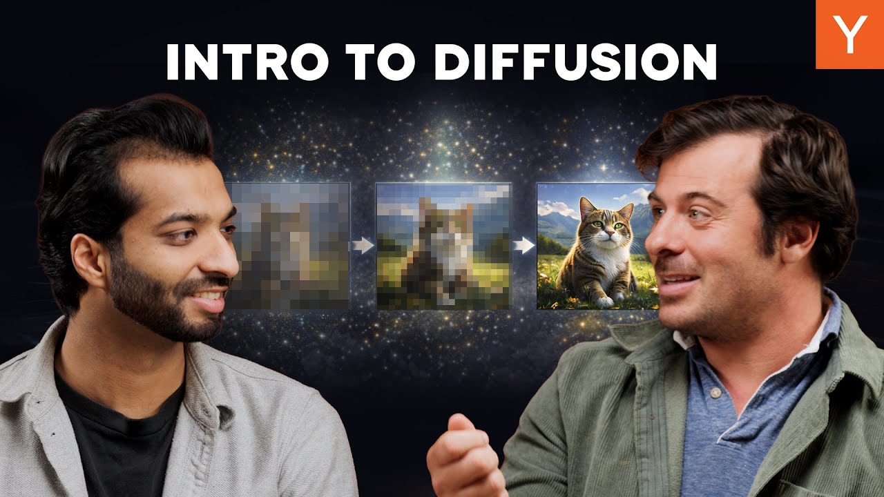
Diffusion is a fundamental machine learning framework designed to learn any data distribution, p(data), for any domain. Its particular strength lies in mapping high-dimensional data to other high-dimensional spaces, even in low-data regimes.

The core process is conceptually a two-step procedure:

1. Forward Process (Noising): Start with a real data sample, like an image, and incrementally add Gaussian noise over a series of timesteps until the original data is completely transformed into random noise. This process is easy to compute.
2. Reverse Process (Denoising): Train a model to reverse this process. The model is given a noised-up sample and a timestep t, and its task is to predict a slightly less noisy version of the data (or the noise itself), eventually reconstructing the original sample from pure noise. This learned denoising model is the final generative tool.

Key Innovations and Evolution

The foundational 2015 paper on non-equilibrium thermodynamics laid out most of the core components, but the field has evolved significantly through a process of “hill climbing” on performance metrics.

• Noise Schedule: A critical component is the schedule by which noise is added. A simple linear interpolation is unstable because the relative amount of error added varies dramatically across timesteps. The goal is to introduce a relatively constant amount of error at each step. This is managed by a “beta schedule” (the rate of diffusion), which creates a non-linear, sigmoid-like curve for how the original image signal is preserved over time. Getting this schedule right is crucial for model stability and performance.

• Loss Function: The objective of the model has been refined to make learning easier.

  • Original Approach: The first models tried to predict the previous, less noisy image, x_{t-1}, by minimizing the KL divergence between the true and learned distributions. The code for this was often complex.
  • Predicting the Error: A key insight was that predicting the noise/error that was added is an easier task for the model than predicting the entire denoised image.
  • Predicting Velocity: An even more effective approach is to predict the “velocity” of the change—the error divided by the time step.

Flow Matching: A Paradigm of Simplicity

Flow matching represents a significant simplification of the diffusion process. Instead of learning a complex, circuitous path to reverse the noising process, flow matching operates on a simpler principle:

There is a global velocity, a straight line, between the noise and the data. The model’s job is to learn this direction, regardless of where it is in the process.

This simplifies the training loop to a few lines of code. For any given time t, you create a noised image x_t by interpolating between the data and a noise sample. The model’s objective is simply to predict the global velocity, which is data - noise. The loss is the mean squared error between the model’s prediction and this target velocity.

# Simplified logic for a training step
x_t = t * data + (1 - t) * noise
velocity = data - noise
prediction = model(x_t, t)
loss = mse_loss(prediction, velocity)

This abstraction is incredibly powerful, as the model can be any architecture (UNET, Transformer) suited for the data type, whether it’s images, protein structures, or weather data. At inference time, the model starts with random noise and iteratively refines it by taking small steps in the direction of the predicted velocity, similar to Euler’s method for solving differential equations.

The “Squint Test” and a Path Toward AGI

When comparing current AI architectures to the human brain (the “squint test”), standard autoregressive Large Language Models (LLMs) fall short. LLMs produce one token at a time, never go backward to revise, and have a staged training process. The brain, in contrast, exhibits massive recursion, continuous learning, and thinks in holistic concepts that are then refined.

Diffusion models align better with this biological blueprint for two key reasons:

1. Leverages Randomness: All of biology and nature utilizes randomness. Diffusion’s core mechanic is the structured leveraging of noise to learn the underlying structure of data, mirroring the stochastic nature of neural processes.
2. Holistic, Iterative Refinement: Diffusion generates an entire output (e.g., an image, a protein structure) at once and iteratively refines it. This is more analogous to human thought, which involves forming a concept and then progressively improving it, rather than building it one character at a time.

Applications and Future Directions

Diffusion is no longer just for images. It has become the state-of-the-art framework across numerous domains, with autoregressive LLMs and game-playing AI (like AlphaGo) being the only major holdouts.

• Media Generation: Images (Midjourney, Stable Diffusion), video (Sora, Veo), and 3D assets.
• Life Sciences: Protein folding (AlphaFold) and small molecule binding.
• Robotics: Learning control policies from demonstrations (Diffusion Policy).
• Science & Engineering: Weather forecasting (Gencast), failure sampling, and more.

For those training models, diffusion should be seriously considered as a fundamental part of the training loop, regardless of the application. For those building products, the rapid, scale-driven improvement in diffusion models suggests that we should expect transformative capabilities in robotics, biology, and other complex fields in the near future.

• Tags:
• Generative AI
• Machine Learning
• AI Research
• Diffusion Models
• Flow Matching
• Denoising