Learned Execution Graphs for Anomaly Detection & Drift in APIs — Ritvik Pandya, JP Morgan Chase

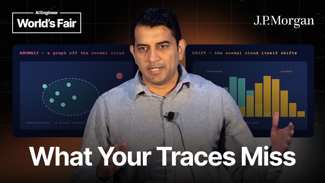
Ritvik Pandya, leading the payments team at JP Morgan, introduced the concept of learn execution graphs for detecting anomalies and drift in high-throughput payment processing systems. The primary goal is to automate detection and significantly reduce manual effort in identifying system issues.

What are Execution Graphs?

Unlike persistent or property graphs, execution graphs are short-lived Directed Acyclic Graphs (DAGs). They represent the holistic processing path of an API request through various middleware steps. This DAG-based representation simplifies understanding the order of service execution, the context passed between nodes, and allows for precise tracking. Even complex scenarios like retries and loops are modeled as distinct entities within the graph to ensure comprehensive tracking.

Tiered Checks and Baselines

The system employs a tiered checking approach, where the execution graph acts as the tier one check. If a request’s execution aligns with its baseline, no further investigation is needed. This is analogous to a simple boarding pass check at an airport. Crucially, baselines are not monolithic; they are per-client and context-specific. For instance, a request from a local client might have a different baseline than one from an external client due to additional checks. This granular baselining helps in significantly reducing false positives.

The core methodology involves:

1. Representing the request processing as a DAG.
2. Establishing a baseline for normal behavior.
3. Detecting deviations from this baseline.
4. Localizing the exact point of deviation within the graph.
5. Comparing the localized issue against predefined thresholds.
6. Taking Action if the deviation exceeds the threshold.

Localizing Performance Problems

One of the key advantages of execution graphs is their ability to pinpoint issues with high precision. Traditional monitoring might report healthy metrics (e.g., low latency, zero errors) even when a mandatory processing step has been silently skipped, reordered, or unexpectedly injected. The graph-based approach immediately flags such structural discrepancies. For example, if a foreign transaction rate service suddenly takes longer, the graph can identify that specific node as the bottleneck, dramatically cutting down root cause analysis time from hours to seconds.

Training the system involves injecting millions of traces over several days (e.g., using OpenTelemetry and StarBench benchmarks) into a benchmark environment to train the anomaly and drift detection models before live deployment.

Anomaly Versus Drift

The talk distinguishes between two types of deviations:

• Anomaly: A one-off, transient incident that deviates from the norm (e.g., a temporary traffic jam extending commute time). The response to an anomaly depends on its criticality.
• Drift: A gradual, sustained shift in pattern that necessitates a re-evaluation and potentially a new baseline (e.g., a permanent increase in commute time due to urban growth, signaling a pattern changed).

The Three Kinds of Drift

Once drift is identified, it can be further categorized:

1. Structural Drift: Occurs when there are changes in the processing flow itself, such as the addition or removal of a node/step. An example given is a coffee shop suddenly adding a

• Tags:
• Distributed Systems
• Feature
• Observability
• Root Cause Analysis
• Anomaly Detection
• OpenTelemetry
• Execution Graphs
• DAGs
• Drift Detection
• Payment Processing
• Baselining
• MTTD Reduction