Graph Neural Networks Explained: A Clear Guide to GNN Basics & Models

An introduction to Graph Neural Networks (GNNs), covering fundamental concepts like nodes, edges, and embeddings. This post delves into the core message-passing mechanism and provides a detailed overview of key architectures including GCN, GraphSAGE, GAT, GIN, and Graph Transformers, explaining their unique approaches and mathematical formulations.

May 25, 2026 5 min read

Graph Neural Networks Explained: A Clear Guide to GNN Basics & Models — source: https://www.youtube.com/watch?v=eGoszzMkGfU

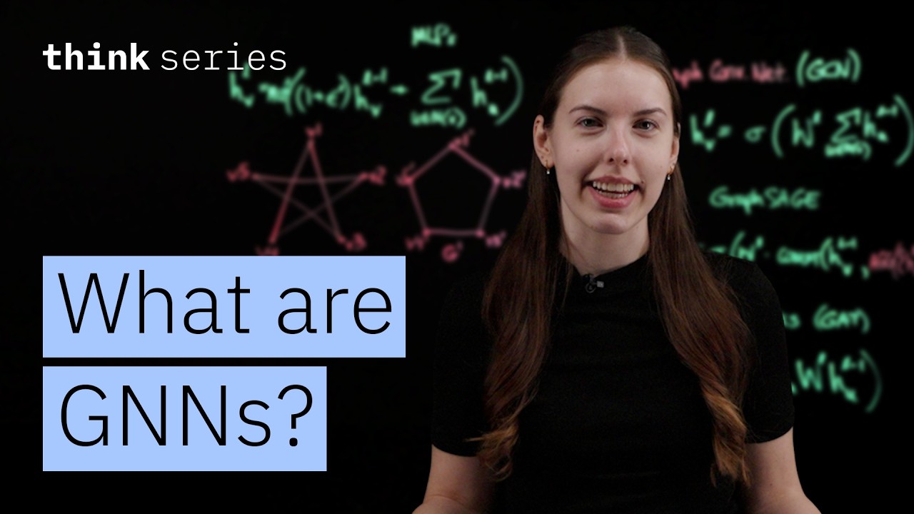
While most machine learning models are designed for structured, tabular data, much of the world’s data is inherently unstructured and interconnected. Graph Neural Networks (GNNs) are a class of models designed specifically to learn from graph-structured data, capturing both the features of entities and the complex relationships that connect them.

Graph Fundamentals

A graph G is a data structure represented by a set of nodes (or vertices) and a set of edges that define connections between the nodes.

Nodes: Entities within the graph.
Edges: The relationships or connections between nodes. Edges can be undirected (a simple connection) or directed (implying a one-way relationship, e.g., “is a student of”).

The connectivity of a graph can be visualized using an Adjacency Matrix, where a non-zero value at (i, j) indicates a connection from node i to node j.

To make graph data usable for machine learning models, we generate embeddings—dense, low-dimensional vector representations that capture the structural and feature-based properties of nodes, edges, or even entire graphs.

Graphs can be categorized as:

Homogeneous: Containing only one type of node and one type of edge.
Heterogeneous: Containing multiple types of nodes and/or edges, such as a graph of students and teachers.

The Core Mechanism: Message Passing

GNNs learn by using a mechanism called message passing, where nodes iteratively exchange information with their neighbors to update their own representations. This process allows the model to learn both local patterns and the global structure of the graph. This happens in layers; with each layer, a node aggregates information from neighbors that are one step further away, enriching its representation.

The message-passing process for a given node typically involves three steps:

Message Creation: Each neighboring node generates a “message,” which is encoded information like its feature vector.
Aggregation: The target node collects all incoming messages and combines them using a permutation-invariant function like sum, mean, max, or an attention-weighted combination.
Update: The node updates its own embedding based on the aggregated message.

Key GNN Architectures

Different GNN architectures implement the message-passing paradigm in unique ways.

Graph Convolutional Networks (GCN)

Inspired by Convolutional Neural Networks (CNNs), GCNs work by aggregating feature representations from a node’s immediate neighbors to create a “smoothed” representation. This makes them a strong choice for tasks like semi-supervised node classification.

The embedding for a node v at layer l is calculated by aggregating the embeddings of its neighbors i from the previous layer (l-1), transforming them with a shared weight matrix W_l, and applying a non-linear activation function σ.

H_v^(l) = σ(W_l * Σ_i(H_i^(l-1)))

GraphSAGE (Graph SAmple and aggreGatE)

GraphSAGE is designed for scalability, especially for massive graphs with millions of nodes. Instead of using a node’s entire neighborhood, it samples a fixed number of neighbors and learns a function to aggregate their information.

The update rule involves aggregating neighbor embeddings, concatenating the result with the node’s own embedding from the previous layer, and then passing it through a weight matrix and activation function.

H_v^(l) = σ(W * concat(H_v^(l-1), aggregate({H_u^(l-1)} for all u in neighbors(v))))

Graph Attention Networks (GAT)

In a GAT, not all neighbors are treated equally. The model uses an attention mechanism to learn the relative importance of different neighbors, assigning higher attention weights (α_vu) to more influential nodes when performing aggregation. These weights are learned during training via backpropagation.

H_v^(l) = σ(Σ_u(α_vu * W * H_u^(l-1)))

Graph Isomorphism Network (GIN)

GIN is one of the most expressive GNN architectures, designed to be as powerful as the Weisfeiler-Lehman (WL) test for graph isomorphism. It excels at distinguishing between different graph structures that simpler GNNs might find indistinguishable. This is critical because standard aggregation methods like mean or max pooling are not injective and can map two different neighborhood structures to the same representation.

Its power comes from a simple but effective update rule that uses a Multi-Layer Perceptron (MLP).

H_v^(l) = MLP((1 + ε) * H_v^(l-1) + Σ_u(H_u^(l-1)))

(Note: ε is a learnable parameter or a fixed scalar.)

Graph Transformers

Extending the highly successful Transformer architecture to graphs, Graph Transformers utilize a global attention mechanism. This allows any node to, in theory, attend to any other node in the graph, making them exceptionally powerful for capturing long-range dependencies.

The process involves several key steps:

Queries, Keys, and Values: The initial node embedding matrix H is projected into three matrices: Query (Q), Key (K), and Value (V).
Attention Score Calculation: Attention scores are computed by comparing each node’s query with every other node’s key. A structural bias term B is added to incorporate graph structure information (e.g., adjacency, distance) into the attention mechanism.
Multi-Head Attention: The attention mechanism is run in parallel with different learned projections (“heads”). The outputs are concatenated and passed through a final projection matrix to combine information from all heads.
Feed-Forward Network (FFN): The output of the attention step is passed through an FFN (typically two linear layers with a ReLU activation) to further refine the representations.
Residual Connections & Layer Normalization: These standard Transformer techniques are used to stabilize training and enable the construction of deeper models.

Summary of Architectures

GCN: Smooths representations by averaging neighbor features.
GraphSAGE: Samples neighbors to enable scalable training on large graphs.
GAT: Focuses on important neighbors using learned attention weights.
GIN: Maximizes expressive power to distinguish between different graph structures.
Graph Transformers: Use global attention for reasoning about long-range dependencies.